The development of corrosion mechanisms is a major issue that industrial experts are faced with while dealing with all phases of metal exploitation.
Damage caused by corrosion affects the increase in both direct and indirect costs of manufacture. With adequate surface protection technology, it is possible to lessen the intensity of corrosion mechanisms’ development. In order for the selected surface protection technology to provide its full protective action, it is necessary to be familiar with its process parameters. This paper deals with a surface protection system that creates a barrier between the aggressive environment and the base material. The tested barrier was created on a base material surface by electrostatic powder spraying. In this experiment, three types of base material (carbon steel, aluminum and galvanized steel) were coated by applying different combinations of operating parameters. Operating parameters, i.e., the voltage and strength of the electric current, were taken as numerical input variables in the experiment. Each experiment design was focused on measuring the thickness of the protective layer. Analysis of the obtained results and statistical data processing confirmed that appropriate parameters (input variables) provided the target thickness of the protective coating on each of the tested materials. Optimization of parameters contributes to the efficiency of production, shortens the processing time and ensures that coating thickness stays within the limits defined either by the manufacturer or the end user.
1. Introduction
In the metal industry, corrosion is probably the most undesired phenomenon that affects all phases of material processing and service life, from the storage of materials up to the construction in the exploitation conditions [1,2,3,4]. If the mentioned issue is presented as a financial cost, dealing with corrosion amounts to USD 2.5 trillion, most of which is spent to alleviate damages caused by corrosion [5,6,7]. In order to minimize such economic losses, it is necessary to choose the most appropriate surface protection for the material exposed to corrosion. Significant savings can be achieved by applying the appropriate technology, whether it concerns changing internal and external damage factors or creating a barrier between the protected material and an aggressive environment. Protection of metals by coating, especially by organic coating, is still the most common surface protection method. It is estimated that three fourths of all metal structures are protected in this way. The barrier created by coating prevents reactants from the environment from penetrating into the base material [8]. Coatings that create a non-conductive protective layer on base materials are commonly used in industries such as the automotive industry, shipbuilding, aviation and aerospace for the protection of tanks and pipelines, etc. [9,10,11,12,13,14]. There are different application procedures and principles determined for certain protection system. This experiment investigates material protection by creating a barrier, which can be achieved by using different technological procedures. One of these is electrostatic powder coating, which provides a protective layer on a base material characterized by good resistance to corrosion and chemicals, as well as by good adhesion properties [15,16]. Adhesion is indicated as a desirable property because no matter how good the individual components of the system are, if adhesion to the base material is poor, the protective potential of the coating will not be fully achieved [17,18]. Besides those positive properties, powder coating is also environmentally friendly, since the coating agent is not diluted during application and does not contain volatile organic solvents. Melting the powder at temperatures of 180–250 °C enables homogeneous, stable and smooth layers to be applied in a thickness of 0.05–1.5 mm to the base material [19,20]. In addition to the mentioned characteristics related to the final appearance of the coating, the success of the powder coating application depends on the process parameters related to voltage and electric current. The position of the spraying gun, i.e., the nozzle from which the powder comes out to the material surface (as shown in Figure 1), is also important. However, in this paper, the authors focused on investigating the influence of the previously mentioned electric current and voltage on the achievement of the target thickness of the protective layer on the base material.
![Figure 1. Position of the nozzle for application of the powder coating to the base material [21].](/images/images/whitepapers/optimizationofpowdercoating/1.jpg)
Figure 1. Position of the nozzle for application of the powder coating to the base material [21].
Proper powder coating requires a high voltage and a low current. In real production conditions, the process of applying a protective coating is often carried out on several types of materials with different conductivity and characteristics, so it is expected that the same process parameters (voltage and current) will not always give the same results regarding the thickness of the applied protective layer. If other parameters, such as the position and movement of the spraying gun, are automatically regulated as a constant, the voltage and electric current can be manipulated to obtain optimal thickness of the coating, which is demanded either by the technical documentation or by the product end user. The objective of this research is to explore the influence that different values of two input variables, i.e., voltage and electric current, have on different materials in order to determine the optimal values that provide the desirable protective layer thickness for each of the tested materials.
2. Experimental Research
The research aims to define the values of voltage and electric current as the input parameters (while keeping other parameters constant) to achieve a desired, i.e., target, thickness of the protective powder-coated layer on the surface of different materials. It is assumed that the powder-coated layer would adhere to the base material differently if the voltage and the electric current used in the process of powder coating differ, so there was a preliminary experiment run to confirm this hypothesis. Except for the varied input variables of the voltage and the electric current, all other parameters during all phases of the powder coating within the preliminary experiment were constant and repeatable. The powder was applied to the material surface by a spraying gun, which operates on a vacuum created by the air flow through the nozzle in the cavity to suck in the powder. The amount of powder taken in depended on the ratio of inlet and added air, which was kept constant, as well as the flow rate, which could also be regulated by additional air.
2.1. Preliminary Experiment
A preliminary experiment was carried out on two types of material: galvanized steel (S235JR + Z) (test mark: PL) and carbon steel (S235) (test mark: UC). The size of the test samples was 150 × 100 mm. The thickness of the powder coating was analyzed to assess its dependence on the varied combinations of current and voltage values, as summarized in Table 1. Electric current and voltage varied between the lower value of 20 and the upper value of 100. The minimum and maximum values of 20 and 100 were chosen for a reason. Namely, by studying the production process in the plant where the experiment was performed, it was observed that all the varied parameter values for different cases always moved within this range. Since no production parameter went below 20 or above 100 (as far as voltage and electric current values are concerned), it was decided to stay within these limits. This range was set because the results of scientific research ultimately have real applications in the production process when it comes to optimizing and selecting operating parameters in accordance with specific job requirements.
Table 1. Values of voltage and electric current in the preliminary experiment.
| Parameters | Galvanized Steel | Carbon Steel |
| U = 20 kV and I = 20 µA | PL1 | UC1 |
| U = 20 kV and I = 100 µA | PL2 | UC2 |
| U = 100 kV and I = 20 µA | PL3 | UC3 |
| U = 100 kV and I = 100 µA | PL4 | UC4 |
The sheets on which the preliminary experiment was performed (Figure 2 and Figure 3) were prepared and pre-treated for powder coating, which was necessary for the achievement of a high-quality protective layer that would be suitable for experimental analysis.
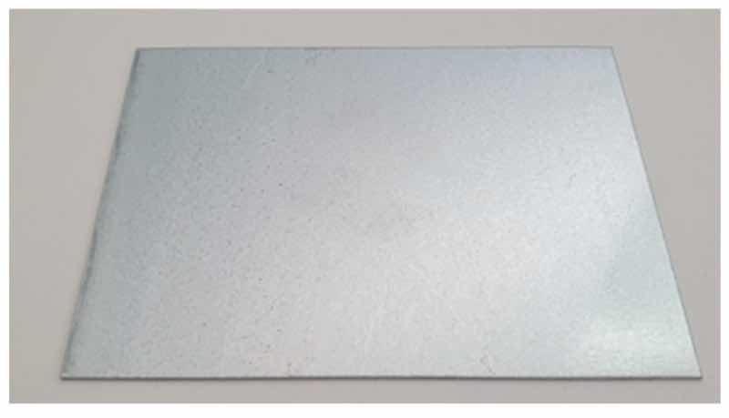
Figure 2. Test sample made out of galvanized steel.
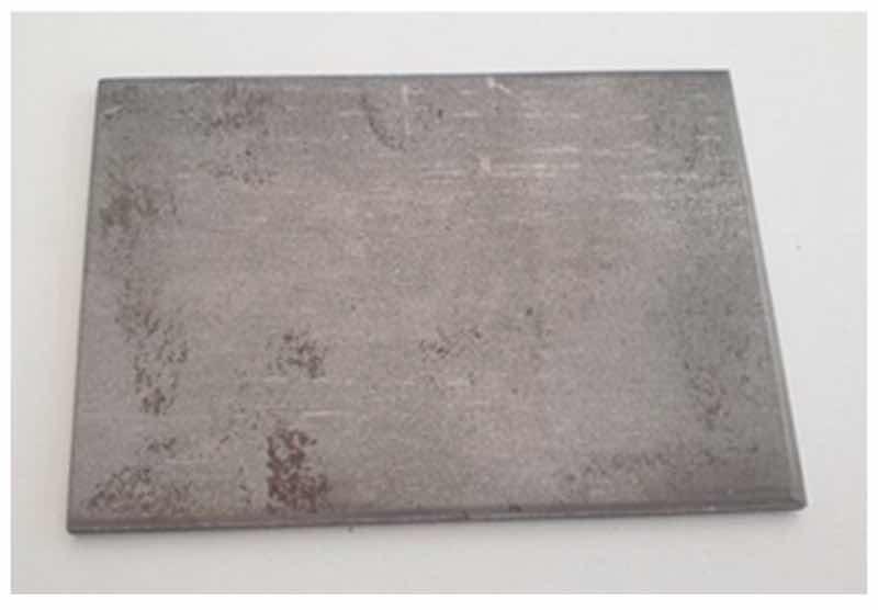
Figure 3. Test sample made out of carbon steel.
Table 2. Results of the preliminary experiment.
| Test Sample | Thickness of the Applied Coating/µm |
| PL1 | 26 |
| PL2 | 14 |
| PL3 | 62 |
| PL4 | 69 |
| UC1 | 23 |
| UC2 | 21 |
| UC3 | 43 |
| UC4 | 78 |
The results of the preliminary experiment indicated clear differences in the thickness of the powder-coated layer when changing the electric current and voltage parameters. Therefore, it was justified to test the stated two parameters as input variables for conducting a detailed experiment in order to determine their optimal values for the achievement of the satisfactory thickness of powder coating on the material surface. Besides galvanized steel (S235JR + Z) and carbon steel (S235), the main experiment was also performed on aluminum (AlMg3).
2.2. Main Experiment and Analysis of Obtained Results
The main experiment was carried out on three different types of material: carbon steel (S235), galvanized steel (S235JR + Z) and aluminum (AlMg3). As in the preliminary test, the size of the test samples was 150 × 100 mm. The research aim was to define the optimal parameters (voltage and strength of electric current) for the application of powder coating in a satisfactory thickness. The coded values of the experiment factors are presented in Table 3. Design-Expert Software 22.0.8 (Stat-Ease, Inc. 1300 Godward Street Northeast, Suite 6400 Minneapolis, MN 55413) was used for experiment planning and statistical data processing.
Table 3. Coded values for the experiment plan.
| Coded Values | Factor 1—Electric Current/µA (Numerical) | Factor 2—Voltage/kV (Numerical) | Factor 3—Material (Categorical) | ||
| –1.414 | 20 | 20 | carbon steel | galvanized steel | aluminum |
| –1 | 31.7157 | 31.7157 | carbon steel | galvanized steel | aluminum |
| 0 | 60 | 60 | carbon steel | galvanized steel | aluminum |
| 1 | 88.2843 | 88.2843 | carbon steel | galvanized steel | aluminum |
| 1.414 | 100 | 100 | carbon steel | galvanized steel | aluminum |
All experiment runs and the results obtained from the measurement of the coating thickness are summarized in Table 4. The presented results refer to the mean value of three repeated measurements for each test sample.
Table 4. Measured coating thickness.
| Test Sample | Experiment Run | Current/µA | Voltage/kV | Material | Coating Thickness/µm |
| 1 | 17 | 31.7157 | 31.7157 | Carbon steel | 36.92 |
| 2 | 22 | 88.2843 | 31.7157 | Carbon steel | 41.82 |
| 3 | 14 | 31.7157 | 88.2843 | Carbon steel | 63.08 |
| 4 | 25 | 88.2843 | 88.2843 | Carbon steel | 77.86 |
| 5 | 5 | 20 | 60 | Carbon steel | 52 |
| 6 | 21 | 100 | 60 | Carbon steel | 68.9 |
| 7 | 30 | 60 | 20 | Carbon steel | 35.4 |
| 8 | 1 | 60 | 100 | Carbon steel | 65.6 |
| 9 | 10 | 60 | 60 | Carbon steel | 72.14 |
| 10 | 3 | 60 | 60 | Carbon steel | 69.94 |
| 11 | 27 | 60 | 60 | Carbon steel | 71.32 |
| 12 | 11 | 31.7157 | 31.7157 | Galvanized steel | 23.5 |
| 13 | 9 | 88.2843 | 31.7157 | Galvanized steel | 28.28 |
| 14 | 4 | 31.7157 | 88.2843 | Galvanized steel | 50.88 |
| 15 | 29 | 88.2843 | 88.2843 | Galvanized steel | 58.4 |
| 16 | 26 | 20 | 60 | Galvanized steel | 48.2 |
| 17 | 12 | 100 | 60 | Galvanized steel | 49.7 |
| 18 | 18 | 60 | 20 | Galvanized steel | 26.3 |
| 19 | 23 | 60 | 100 | Galvanized steel | 55 |
| 20 | 15 | 60 | 60 | Galvanized steel | 52.58 |
| 21 | 28 | 60 | 60 | Galvanized steel | 47.48 |
| 22 | 7 | 60 | 60 | Galvanized steel | 52.4 |
| 23 | 33 | 31.7157 | 31.7157 | Aluminum | 27.4 |
| 24 | 20 | 88.2843 | 31.7157 | Aluminum | 38.46 |
| 25 | 2 | 31.7157 | 88.2843 | Aluminum | 59 |
| 26 | 24 | 88.2843 | 88.2843 | Aluminum | 68.72 |
| 27 | 6 | 20 | 60 | Aluminum | 49.3 |
| 28 | 13 | 100 | 60 | Aluminum | 55.4 |
| 29 | 32 | 60 | 20 | Aluminum | 24.2 |
| 30 | 31 | 60 | 100 | Aluminum | 57.6 |
| 31 | 16 | 60 | 60 | Aluminum | 63.34 |
| 32 | 8 | 60 | 60 | Aluminum | 57.08 |
| 33 | 19 | 60 | 60 | Aluminum | 62.98 |
Figure 4 shows the measurement of the thickness of the applied layer (SaluTron ComBi D1000, SaluTron Messtechnik GmbH, Dr.-Gottfried-Cremer-Allee 30/7, D-50226 Frechen) on the test sample. The measurement of the thickness of the applied layer was carried out by measuring the thickness of the applied layer at fifteen different locations on each test sample. Of all the measured values, the mean value of all measurements on each sample was recorded as the reference value for the planned experiment output (output variable).
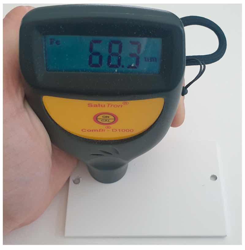
Figure 4. Measuring the thickness of the applied protective layer.
Within this experiment, results were obtained by calculating the arithmetic mean of three repeated measurements. When performing the experiment, the principle of randomization was applied, so the samples were processed in a random order, as presented in Table 4. According to the results, the application of the coating was carried out first on test sample 8 (experiment run 1), while sample 23 (experiment run 33) was the last one to be coated. Analysis of the experimental research results (Table 4) showed that the minimum response value (coating thickness) was 23.5 µm, while the maximum was 77.86 µm. The arithmetic mean of the response in this case was 51.85 µm.
Referring to the data obtained for the thickness of the powder-coated layer (Table 4), testing of the linear model, the linear model with second-order interaction 2FI, the quadratic model and the cubic model confirmed that the quadratic model was the best, as presented in Table 5. The model was tested in relation to the p-value (mean square deviation), p-value for deviation from the model and coefficients of determination (coefficient of determination, adjusted coefficient of determination and predicted coefficient of determination).
Table 5. Simulation of four models in the Design-Expert software—coating thickness.
| Model | Mean Square Deviation p-Value | Deviation from the Model p-Value | Coefficient of Determination | Adjusted Coefficient of Determination | Predicted Coefficient of Determination |
| Linear | <0.0001 | 0.0039 | 0.7632 | 0.7294 | 0.6826 |
| 2FI | 0.9600 | 0.0023 | 0.7730 | 0.6842 | 0.5764 |
| Quadratic | <0.0001 | 0.1275 | 0.9557 | 0.9325 | 0.8823 |
| Cubic | 0.0376 | 0.3634 | 0.9845 | 0.9618 | 0.8748 |
The p-value (probability) for the F variable for the model is less than 0.05, indicating that at least one of the 11 regression variables has a non-zero regression coefficient, i.e., the contribution to the model is significant. The coefficient of determination R2, 0.9557, is the proportion of explained variability to the total variability. However, a higher value of the coefficient of determination does not necessarily mean that the regression model is good. If new terms are added to the model, the R2 value will increase, regardless of whether the added term is statistically significant or not. Therefore, there is a possibility that models with a high coefficient of determination poorly express the estimate of the new value or the arithmetic mean of the response. Because the R2 value increases with the addition of new terms to the model, the adjusted coefficient of determination R2adj is also used, which is adjusted for the number of model terms in relation to the number of experimental conditions [22]. The adjusted coefficient of determination R2adj, adjusted for the number of model terms in relation to the number of experimental conditions, is 0.9325. The value of the adjusted coefficient of determination will not always increase with the inclusion of new variables in the model. On the contrary, the addition of new insignificant variables will decrease the aforementioned value. A significant difference between R2 and R2adj indicates that insignificant terms are very likely included in the model [22]. The predicted coefficient of determination R2pred is 0.8823. Since, with the largest coefficient of determination R2, the difference between R2adj and R2pred is not greater than 0.2, the choice of this quadratic model is justified. Table 6 contains a report obtained from the Design-Expert software for the quadratic model. The dependence of the coating thickness on the input variables in the experiment is shown by the quadratic model.
Table 6. Analysis of variance of the regression model for coating thickness.
| Source | Sum of Squares | Number of Degrees of Freedom | Mean Square Deviation | Value of the F-Test | p-Value |
| Model | 6987.22 | 11 | 635.20 | 41.20 | <0.0001 |
| A—Current | 318.34 | 1 | 318.34 | 20.65 | 0.0002 |
| B—Voltage | 4058.39 | 1 | 4058.39 | 263.21 | <0.0001 |
| C—Material | 1203.26 | 2 | 601.63 | 39.02 | <0.0001 |
| AB | 10.60 | 1 | 10.60 | 0.6877 | 0.4163 |
| AC | 53.15 | 2 | 26.58 | 1.72 | 0.2027 |
| BC | 7.72 | 2 | 3.86 | 0.2502 | 0.7809 |
| A2 | 248.87 | 1 | 248.87 | 16.14 | 0.0006 |
| B2 | 1306.79 | 1 | 1306.79 | 84.75 | <0.0001 |
| Residual | 323.79 | 21 | 15.42 | ||
| Lack of Fit | 279.86 | 15 | 18.66 | 2.55 | 0.1275 |
| Pure Error | 43.93 | 6 | 7.32 | ||
| Cor Total | 7311.01 | 32 |
The sum of squares total is the total variation of the value 7331.01. The number of degrees of freedom (df) is 32 (number of data in the experiment: 33 − 1 = 32). The sum of squares residual is the unexplained variance, a random error, with a residual of 323.79. The number of degrees of freedom for the residual is 21 (number of data minus the number of model members minus 1: 33 − 11 − 1 = 21). The mean square residual is 15.42. The sum of squares model is the explained variance, which is 6987.22. The number of degrees of freedom for the model is 11 (11 regression variables). The mean square deviation for the regression model has a value of 635.20. The members of the model A, B, C, A2 and B2 are significant in the model (the probabilities for the F variables whose values are 20.65, 263.21, 39.02, 16.14 and 84.75 have p-values less than 0.05). The other members of the model AB, AC and BC are not significant (the probabilities for the F variables whose values are 0.6877, 1.72 and 0.2502 have p-values greater than 0.05). The value of the model deviation (lack of fit) is presented here with a probability for the F variable of 0.1275, which indicates that the model’s estimate of reality is good. The unbiased estimate of the variance is the mean square deviation of the residual, which is 15.42, while the standard error (deviation) is the root of the variance and is 3.9268.
Expression 1 describes the regression model for the dependence of coating thickness on the input variables (Factor A—current, Factor B—voltage, Factor C—material). The values of the mentioned variables are coded for high factor levels as +1 and for low factor levels as –1, according to Table 3. Expression 2 describes a regression model with actual factor values, where factor C (material) is carbon steel. Expression 3 refers to a regression model with actual factor values, where factor C is galvanized steel, and expression 4 refers to a regression model with actual factor values, where factor C is aluminum.
Coating thickness = 61.03 + 3.64 × A + 13.00 × B + 7.69 × C1 − 7.06 × C2 + 0.9400 × AB + 1.81 × AC1 − 1.84 × AC2 + 0.1098 × BC1 − 0.7428 × BC2 − 3.83 × A2 − 8.78 × B2 (1)
Coating thickness = −23.19563 + 0.697016 × Current + 1.71055 × Voltage + 0.001175 × Current × Voltage − 0.004791 × Current2 − 0.010978 × Voltage2 (2)
Coating thickness = −28.40584 + 0.568151 × Current + 1.68041 × Voltage + 0.001175 × Current × Voltage − 0.004791 × Current2 − 0.010978 × Voltage2 (3)
Coating thickness = −28.86534 + 0.634377 × Current + 1.72905 × Voltage + 0.001175 × Current × Voltage − 0.004791 × Current2 − 0.010978 × Voltage2 (4)
Figure 5, Figure 6 and Figure 7 provide graphic presentations of the models, showing how the coating thickness behaves when influenced by changes in current and voltage. The dependence of the coating thickness on the input parameters is shown by the figures below when the coating is applied to carbon steel (Figure 5), galvanized steel (Figure 6), and aluminum (Figure 7).
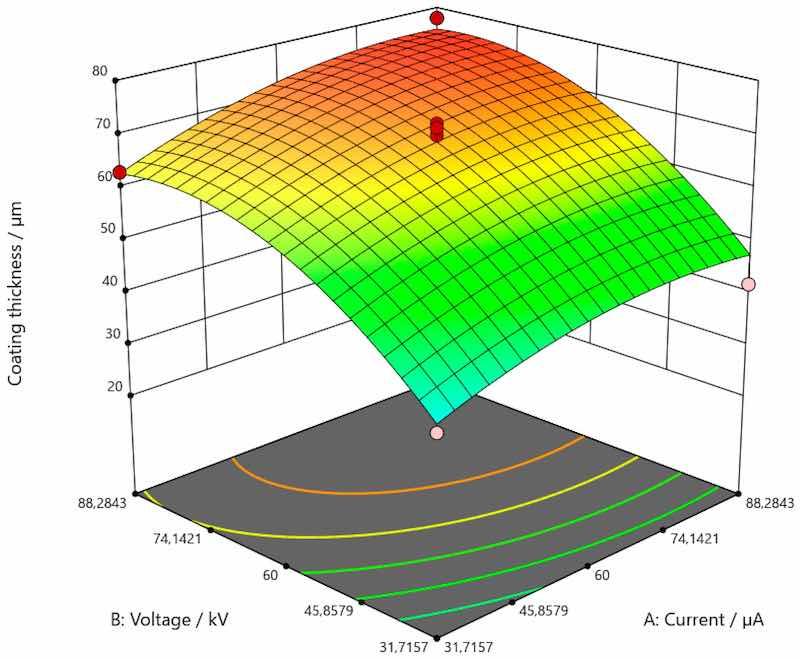
Figure 5. Response surface for the regression model of the dependence of coating thickness for carbon steel.
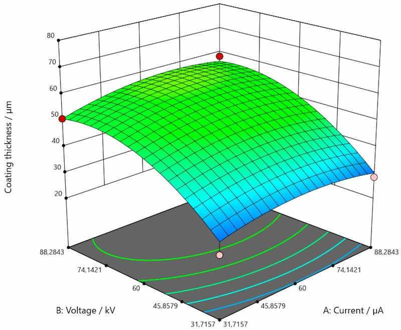
Figure 6. Response surface for the regression model of the dependence of coating thickness for galvanized steel.
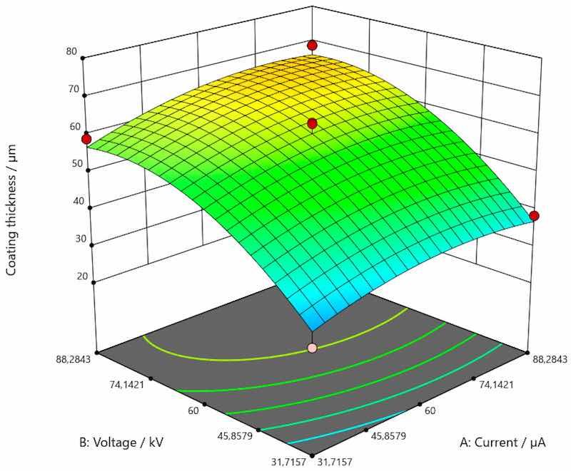
Figure 7. Response surface for the regression model of the dependence of coating thickness for aluminum.
As shown in Figure 5, there was a trend of increase in the value of coating thickness along with the increase of current and voltage for the coating applied on carbon steel. Figure 6 shows the trend of increasing coating thickness values with increasing voltage for all current values when the coating is applied to galvanized steel. More precisely, coating thickness remains the same if the current and voltage are 31.7157 and 88.2834 µA. When the voltage is increased, the coating thickness increases as well. As presented by Figure 7, an increase in the value of coating thickness occurs with the increase of current and voltage when the coating is applied on aluminum.
Table 7 illustrates the values for standard error of regression coefficients and the lower and upper limits of the confidence interval (CI).
Table 7. Standard errors of regression coefficients—coating thickness.
| Factor | Coefficient Estimate | Number of Degrees of Freedom | Standard Error | 95% CI Low | 95% CI High |
| Independent variable | 61.03 | 1 | 1.31 | 58.31 | 63.75 |
| A—Current | 3.64 | 1 | 0.8015 | 1 98 | 5.31 |
| B—Voltage | 13.00 | 1 | 0.8015 | 11.34 | 14.67 |
| C [1] | 7.69 | 1 | 0.9667 | 5.68 | 9.70 |
| C [2] | −7.06 | 1 | 0.9667 | −9.07 | −5.05 |
| AB | 0.9400 | 1 | 1.13 | −1.42 | 3.30 |
| AC [1] | 1.81 | 1 | 1.13 | −0.5518 | 4.16 |
| AC [2] | −1.84 | 1 | 1.13 | −4.20 | 0.5180 |
| BC [1] | 0.1098 | 1 | 1.13 | −2.25 | 2.47 |
| BC [2] | −0.7428 | 1 | 1.13 | −3.10 | 1.61 |
| A2 | −3.83 | 1 | 0.9540 | −5.82 | −1.85 |
| B2 | −8.78 | 1 | 0.9540 | −10.77 | −6.80 |
Model adequacy checking is an important part of the data analysis procedure. It is necessary to test the estimated regression model in order to determine with certainty that the specified model is a high-quality approximation of the real process and to check, i.e., to prove, that all assumptions are valid when using the least squares method.
When checking the adequacy of the regression model, one of the most important assumptions is that the errors in the model (residuals) should be independent and distributed normally, with expected zero and variance ϭ2.
Figure 8, Figure 9 and Figure 10 present the diagrams by the means of which the model adequacy was checked.
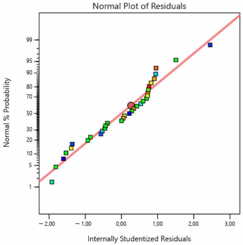
Figure 8. Checking the assumption on normal distribution—coating thickness.
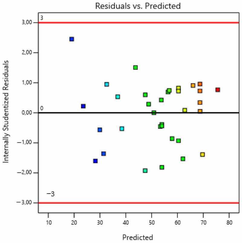
Figure 9. Residuals—predicted values—coating thickness.
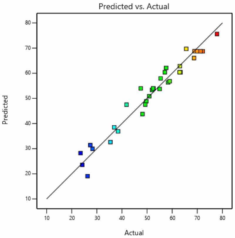
Figure 10. Actual and predicted value—coating thickness.
As seen in Figure 8, residuals (i.e., internally studentized residuals—transformed or scaled residuals) were distributed normally, since there were no significant deviations from the line. Figure 9 shows that errors, i.e., residuals, did not correlate (there was neither negative nor positive correlation) with certain values and that they did not exceed the diagram boundaries in values of ±3. The points in the diagram are colored according to the response (coating thickness). Figure 10 presents both the actually measured values and the values predicted by the model.
Based on the above-presented research results, it is possible to optimize the input parameters (current and voltage) in order to obtain the target value of an output (thickness of applied coating) for each of the tested materials. Table 8 gives an overview of the limitations set for each of the input parameters, as well as the target value of the coating thickness. Table 9 contains the optimal values of input parameters for achieving target coating thickness on carbon steel, galvanized steel and aluminum.
Table 8. Limitations for optimization of parameters for carbon steel coating.
| Input Parameter | Goal | Lower Limit | Upper Limit |
| Current/µA | in range | 20 | 100 |
| Voltage/kV | in range | 20 | 100 |
| Coating thickness/µm | ≈60 µm |
Table 9. Optimal solution for the achievement of target thickness of the powder-coated layer.
| Current/µA | Voltage/kV | Material | Coating Thickness/µm |
| 74.813 | 43.984 | carbon steel | 60 |
| 69.150 | 80.236 | galvanized steel | 58.644 |
| 98.405 | 63.420 | aluminum | 60 |
The optimal solution, i.e., optimal values, of the input parameters (current and voltage) for the achievement of the target thickness of the coating on carbon steel is presented in Figure 11, on galvanized steel in Figure 12 and on aluminum in Figure 13.
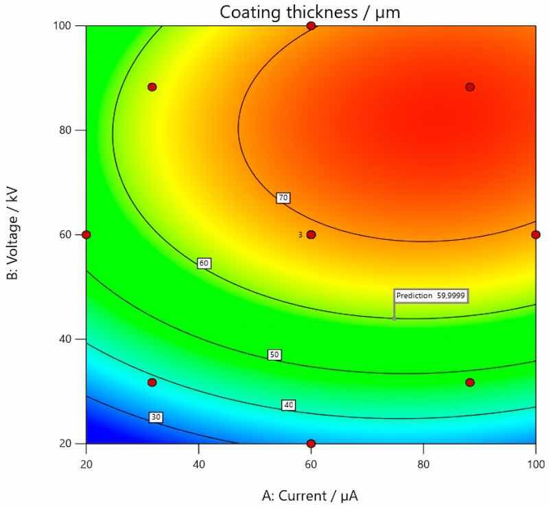
Figure 11. Optimal values of input parameters for the achievement of target thickness of coating on carbon steel.
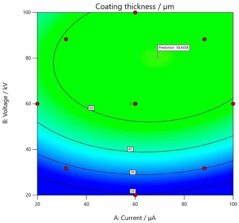
Figure 12. Optimal values of input parameters for the achievement of target thickness of coating on galvanized steel.
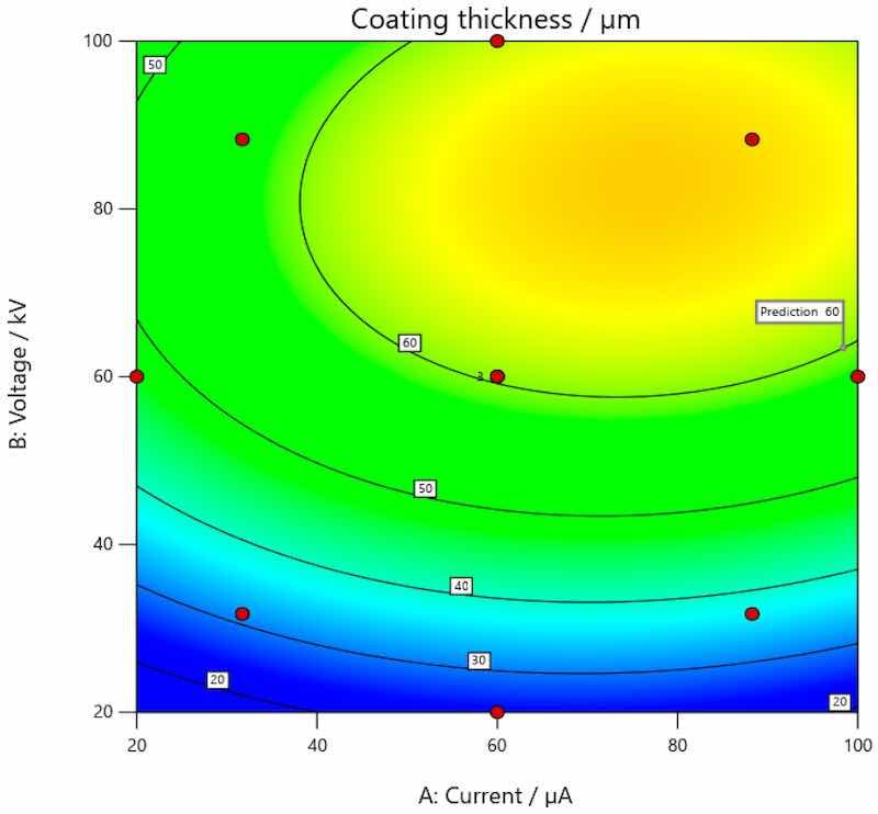
Figure 13. Optimal values of input parameters for the achievement of target coating thickness on aluminum.
The analysis of the research results obtained within this experiment confirmed that voltage and current have a great influence on the thickness of the coating. This hypothesis was already confirmed in the preliminary experiment, within which only combinations of limited values were examined. The more comprehensive effect of their interaction was examined in the main experiment. The conducted research thus provides insight into how important the implementation of a scientific approach is in all segments of production processes. Namely, the individual effect of certain process parameters that are defined here as input variables is very easy to verify; however, what is also extremely important is the interaction of individual parameters and their effects. By using software for experimental planning and statistical data processing, the interaction effect of all input variables of the planned experiment on the output variable (coating thickness) was clearly demonstrated. As previously mentioned, in preliminary research using classical methods and a simple experimental plan, it is only possible to observe that certain changes can result in varying combinations of parameters. However, with more detailed analysis and processing, it is possible to arrive at mathematical models with which it is possible to assess cause-and-effect relationships; it is also possible to perform additional analyses of the collected data in order to define the optimal values of individual parameters that will result in the desired values and characteristics of the individual observed property. In this way, we delve into the very principles of achieving, in this case, coatings of the desired thicknesses and obtain a clearer picture of the process itself. From this, it is possible to further speed up and improve the production processes themselves. Graphic presentations, as in Figure 5, Figure 6 and Figure 7, show how coating thickness changes on different base materials (carbon steel, galvanized steel and aluminum) when influenced by the input variables. It is interesting that this type of analysis and data processing led to the determination of optimal values of voltage and current that provide a certain thickness of the coating. Coating manufacturers recommend the thickness in which the coating should be applied; the thickness of coating can also be requested by the end user of a coated product. Since coating is applied on different materials, it is clear that the same combination of parameters (current and voltage) will not always result in the same thickness of applied coating. Therefore, defined mathematical models and the possibility of optimization as presented in this paper can speed up the whole process of coating application. The targeted, i.e., desired, coating thickness in this research was 60 µm. Statistical analysis and subsequent optimization of the observed process parameters proved that the target coating thickness on carbon steel can be achieved by setting the current to approximately 74.813 µA and the voltage to 43.984 kV. In order to achieve the target coating thickness on galvanized steel, the optimal current would be 69.150 µA and voltage is 80.236 kV, while the same parameters applied on the coating of aluminum would be 98.405 µA and 63.420 kV, respectively.
3. Conclusions
In order to prevent the development of corrosion mechanisms, appropriate surface protection technology should be applied to base materials. The full protective potential of the applied coating depends on the optimal selection of the application process parameters. The influence of voltage and current on the thickness of the applied coating is elaborated in this paper through the statistical processing of the obtained experimental data. The influence of the observed parameters also depends on the type and characteristics of the base material.
Manufacturers of protective coating systems, in this case, powder coatings, usually recommend values for the thickness of the applied layer, which depend on the coating properties. Besides coatings manufacturers, the end users of a coated product may also have special requirements regarding coating thickness. As proven by this research, statistical data analysis, definition of mathematical models and optimization of process parameters ensure that the coating thickness stays within acceptable limits. A validation experiment was conducted based on the optimal process parameters thus generated. A protective coating was applied to each of the observed base materials with the optimal application parameters recommended by the software analysis, and it was observed that the desired properties in terms of coating thickness corresponded to the set conditions. In this way, it is possible to speed up the whole process of determining the operating parameters and to efficiently achieve the demanded values of protective coatings.
Written by Tomislav Šolić1, Dejan Marić1, Ivan Peko2, and Ivan Samardžić1 1: Mechanical Engineering Faculty in Slavonski Brod, University of Slavonski Brod, Trg I. B. Mažuranić 2, 35000 Slavonski Brod, Croatia; 2: Faculty of Science, University of Split, Ruđera Boškovića 33, 21000 Split, Croatia
Author Contributions: Conceptualization, T.Š. and D.M.; methodology, T.Š.; software, D.M.; validation, I.P.; formal analysis, D.M.; investigation, T.Š., D.M. and I.P.; resources, I.S.; data curation, I.S.; writing—original draft preparation, T.Š. and I.P.; writing—review and editing, T.Š. and I.P.; visualization, I.P.; supervision, I.S. All authors have read and agreed to the published version of the manuscript.
Funding: This research received no external funding.
Conflicts of Interest: The authors declare no conflicts of interest.
References
Montoya, L.F.; Contreras, D.; Jaramillo, A.F.; Carrasco, C.; Fernández, K.; Schwederski, B.; Rojas, D.; Melendrez, M.F. Study of anticorrosive coatings based on high and low molecular weight polyphenols extracted from the Pine radiata bark. Prog. Org. Coat. 2019, 127, 100–109. [Google Scholar] [CrossRef]
Dariva, C.G.; Galio, A.F. Corrosion Inhibitors—Principles, Mechanisms and Applications. In Developments in Corrosion Protection; Intech: London, UK, 2014; pp. 365–380. [Google Scholar]
Chen, B.-Q.; Zhang, X.C. Guedes Soares: The effect of general and localized corrosion on the collapse pressure of subsea pipelines. Ocean. Eng. 2022, 247, 110719. [Google Scholar] [CrossRef]
Shojai, S.; Schaumann, P.; Braun, M.; Ehlers, S. Influence of pitting corrosion on the fatigue strength of offshore steel structures based on 3D surface scans. Int. J. Fatigue 2022, 164, 107128. [Google Scholar] [CrossRef]
Okyere, M.S. Corrosion Protection for the Oil and Gas Industy: Pipelines, Subsea Equipment, and Structures; CRC Press: Boca Raton, FL, USA; Taylor & Francis Group: Abingdon, UK, 2019; p. 169. [Google Scholar]
NACE International. International Measures of Prevention, Application, and Economics of Corrosion Technologies Study; NACE International: Houston, TX, USA, 2016; p. 72. [Google Scholar]
Li, J.; He, J.; Chisholm, B.J.; Stafslien, M.; Battocchi, D.; Bierwagen, G.P. An investigation of the effects of polymer binder compositional variables on the corrosion control of aluminum alloys using magnesium-rich primers. J. Coat. Technol. Res. 2010, 7, 757–764. [Google Scholar] [CrossRef]
Šolić, T.; Marić, D.; Novoselović, D.; Samardžić, I. Optimization of Parameters for Protection of Materials by Primer Application. Coatings 2022, 12, 413. [Google Scholar] [CrossRef]
Chang, C.-H.; Huang, T.-C.; Peng, C.-W.; Yeh, T.-C.; Lu, H.-I.; Hung, W.-I.; Weng, C.-J.; Yeh, J.-M. Novel anticorrosion coatings prepared from polyaniline/graphene composites. Carbon 2012, 50, 5044–5051. [Google Scholar] [CrossRef]
Chang, K.-C.; Ji, W.-F.; Lai, M.-C.; Hsiao, Y.-R.; Hsu, C.-H.; Chuang, T.-L.; Wei, Y.; Yeh, J.-M.; Liu, W.-R. Synergistic effects of hydrophobicity and gas barrier properties on the anticorrosion property of PMMA nanocomposite coatings embedded with graphene nanosheets. Polym. Chem. 2013, 5, 1049–1056. [Google Scholar] [CrossRef]
Ding, J.; Rahman, O.U.; Peng, W.; Dou, H.; Yu, H. A novel hydroxyl epoxy phosphate monomer enhancing the anticorrosive performance of waterborne graphene/epoxy coatings. Appl. Surf. Sci. 2018, 427, 981–991. [Google Scholar] [CrossRef]
Javidparvar, A.A.; Ramezanzadeh, B.; Ghasemi, E. Effect of Various Spinel Ferrite Nanopigments Modified by Amino Propyl Trimethoxy Silane on the Corrosion Inhibition Properties of the Epoxy Nanocomposites. Corrosion 2016, 72, 761–774. [Google Scholar] [CrossRef] [PubMed]
Yang, W.; Xu, D.; Wang, J.; Yao, X.; Chen, J. Microstructure and corrosion resistance of micro arc oxidation plus electrostatic powder spraying composite coating on magnesium alloy. Corros. Sci. 2018, 136, 174–179. [Google Scholar] [CrossRef]
Zhang, T.; Zhang, T.; He, Y.; Wang, Y.; Bi, Y. Corrosion and aging of organic aviation coatings: A review. J. Aeronaut. 2023, 36, 1–35. [Google Scholar] [CrossRef]
Zhnag, J.; Kong, G.; Li, S.; Le, Y.; Che, C.; Zhang, S.; Lai, D.; Liao, X. Graphene-reinforced epoxy powder coating to achieve high performance wear and corrosion resistance. J. Mater. Res. Technol. 2022, 20, 4148–4160. [Google Scholar] [CrossRef]
Barletta, M.; Gisario, A.; Rubino, G. Scratch response of high-performance thermoset and thermoplastic powders deposites by the electrostatic spray and ‘hot dipping’ fluidised bed coating methods: The role of the contact condition. Surf. Coat. Technol. 2011, 205, 5186–5198. [Google Scholar] [CrossRef]
Mariappan, T.; Kamble, A.; Naik, S.M. An investigation of primer adhesion and topcoat compatibility on the waterborne intumescent coating to structural steel. Prog. Org. Coat. 2019, 131, 371–377. [Google Scholar] [CrossRef]
Puspitasari, W.C.; Ahmad, F.; Ullah, S.; Hussain, P.; Megat-Yusoff, P.S.M.; Masset, P.J. The study of adhesion between steel substrate, primer, and char of intumescent fire retardant coating. Prog. Org. Coat. 2019, 127, 181–193. [Google Scholar] [CrossRef]
Esih, I. Osnove Površinske Zaštite; Fakultet Strojarstva i Brodogradnje: Zagreb, Hrvatska, 2010. [Google Scholar]
Juraga, I.; Alar, V.; Stojanović, I. Korozija i Zaštita Premazima; Fakultet Strojarstva i Brodogradnje: Zagreb, Hrvatska, 2014; p. 186. [Google Scholar]
Ye, Q.; Domnick, J. On the simulation of space charge in electrostatic powder coating with a corona spray gun. Powder Technol. 2003, 135, 250–260. [Google Scholar] [CrossRef]
Montgomery, D.C. Design and Analysis of Experiments, 9th ed.; John and Wiley and Sons: Hoboken, NJ, USA, 2017. [Google Scholar]


